Appendix G: Numerical evaluation of wavefunction boundary integrals

Boundary methods are a central component of this thesis. Closed integrals of a function $f{({\mathbf s})}$ over the boundary coordinate ${\mathbf s}$ are ubiquitous. Generally $f{({\mathbf s})}= g{({\mathbf s})}h{({\mathbf s})}$ and a square matrix $F$ of integrals

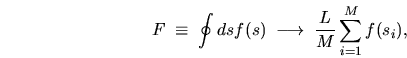
$$F_{nm} \; = \; \oint d{\mathbf s}\, g_n{({\mathbf s})}h_m{({\mathbf s})}, \hspace{1in} n,m \; = \; 1 \cdots N ,$$ (G.1)

is required, where the indices label multiple functions. For evaluation of the quantum band profile (Chapters 2 and 3), the local density of states (Chapter 6), the tension and area-norm matrices (Chapter 5), and the Vergini matrix and its derivative (Chapter 6), $g{({\mathbf s})}$ and $h{({\mathbf s})}$ are basis functions or eigenstates which oscillate about zero on the length scale $\lambda_{{\mbox{\tiny B}}}$, the quantum (de Broglie) free-space wavelength. The deformation function boundary integrals (Chapter 4) do not involve any quantum scale, but are also evaluated using the method below. I will present only the $d=2$ case where boundary integrals over ${\mathbf s}$ become line integrals over $s$; the generalization to higher $d$ is simple.

My tool for evaluation of an integral on a closed curve is the discretization

$$F \; \equiv \; \oint ds f(s) \; \longrightarrow \; \frac{L}{M} \sum_{i=1}^M f(s_i) ,$$ (G.2)

where $L$ is the range of $s$, that is, the length of the line integral (billiard perimeter). The $M$ points are spread uniformly (equidistant in $s$) along the closed curve. Because no point is special, no special quadrature [161] weights arise near any endpoints: all weights are equal. More sophisticated and accurate approximations exist for closed line integral evaluation [58], however this is sufficient for my needs and is very simple to code. Its errors will be discussed and tested below.

A single integral (G.2) requires $M$ function evaluations of $f$. Naively one might guess that filling a matrix $F$ using (G.1) requires $O(N^2M)$ evaluations. However, the correct way to compute (G.1) requires only $O(NM)$ such evaluations: First fill the rectangular matrices $G_{im} = g_m(s_i)$ and $H_{im} = h_m(s_i)$, from which follows

$$F \; = \; \frac{L}{M} G^{{\mbox{\tiny T}}} H .$$ (G.3)

This matrix multiplication does require $N^2M$ operations, but being simple adds and multiplications (and using optimized library code e.g. BLAS), it is very fast and does not affect the scaling. If you like, the matrix multiply `performs' the integration over $i$. In the case where $g$ and $h$ are the same function, only $NM$ evaluations are required. Note that if a general weighting function $w{({\mathbf s})}$ is required in the integrand (G.1), it can easily be incorporated into $G$ or $H$, or equivalently be included as a diagonal matrix $W$ inserted between $G^{{\mbox{\tiny T}}}$ and $H$ in (G.3).