Resources Math 3 Course Home Page Math 3 Course Syllabus Practice Exams Textbook Home Page Post a Comment

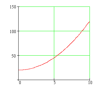
Contents In this lecture we learn to draw the slope field of a differential equation, and consider a simple procedure, called "Euler's Method," for finding numerical (approximate) solutions. We also develop the case study for this segment (lectures 17-20) of our calculus course, Population Modeling. Quick Question Could this graph model the number of rabbits in a pen of fixed size and fixed daily allotment of food over a ten-year period? Answer Outline Outlines for Slope Fields and Euler's Method Case Study: Population Modeling Textbook Slope Fields and Euler's Method Case Study: Population Modeling Today's Homework Log into WebWorK Quiz Slope Fields and Euler's Method Quiz Case Study: Population Modeling Quiz Examples An investor has a savings account that pays 3.5% interest. The investor opens the account with $500 and makes an additional deposit of $500 at the end of each year. Assume the function S(t), which gives the amount in the savings account after t years, satisfies a given the differential equation. Use Euler's method to estimate the amount in the account at the end of 5, 10, and 25 years, using a step size of 0.1. Let y be a function of x that satisfies a given differential equation. Use Euler's method with step sizes .01, .001, .0001 to estimate the value of y when x = .99. Do these estimates seem reliable? Assume that the point (−1, .001) is on the graph of a function that satisfies a given differential equation. Estimate the value of y when x = 1 using Euler's method. Match three differential equations to their slope fields. Suppose we want to model the growth of a bacteria colony. We know that the rate of change of the population (P) is directly proportional to the population. Early observations suggest that they are in fact equal. If the initial population is 100, use Euler's method with stepsize = 0.1 to predict the population in 6 hours. After three hours, we observe the bacteria colony and find the population is now 1600. Use this information to solve the differential equation in the previous example, and find a more accurate constant of proportionality. How does this model differ from the previous one? Again, predict the population at t = 6 hours and compare with the previous estimate. More research indicates that the growth of the bacteria colony is proportionally dependent on the amount of oxygen available. In the controlled environment where our sample resides, all the oxygen will be exhausted in 3 days (72 hours). Thus, our new differential equation modeling the bacteria growth is dP/dt = k P (72 − t)/72. Determine the population at time t = 6 hours, and describe the long term behavior of the bacteria colony. Applets Euler's Method Euler Population Predictions Videos Use Euler's Method to solve y′ = xy Solve dw/dt = k(1 - w/m) to model population of weeds in a garden

Lecture 18 | Index | Lecture 20